End of the Year

We hope you did great on the exam. Our whole team thanks you for keeping up with our blog. If you have any comments on how we can improve this "classroom blog" for next year, please feel free to comment below!

Review: Divergence Theorem + Stokes' Theorem

Today we did some review on the Divergence Theorem and Stokes' Theorem. These problems intertwined the various concepts we have been learning, and learned to switch between formulas to get the most convenient equation to solve. Test on Friday!!!

How do we apply Stoke's Theorem?

So we learned the last theorem ever in this course today-- Stokes' Theorem. Just as magnificent as Mr. Honner made the theorem sound, it is actually pretty amazing. It basically incorporates both the Divergence Theorem and Green's Theorem into one. It states:

Let S be a smooth surface that is bounded by a simple closed curve. Then the closed integral of F dot dr is equal to the double integral of curl F dot dS, over the surface S.

In the Divergence Theorem, surface integrals and triple integrals are shown to be interrelated and it shows the flux. Green's Theorem relates line integrals (work) and double integrals. But in this theorem, it links the two theorems--surface integrals and line integrals, which makes it pretty cool.

Well, that was the last theorem you'll ever learn in this course. Make use of it on the final on Friday!

The homework for tonight was the same as yesterdays: P. 1130 # 2, 5, 8, 10, 25, 26.

How do we compute flux?

Today we went over evaluating SSs f(x,y) ds some more, and then learned another integral: the flux integral. The integral is SS F dot n ds. This eventually gives us the following, more practical equations:
1) SSd F dot (-Gxi-Gyk+k)dA
2) SSd F dot (Ru x Rv) dA

Using these integrals, you can evaluate the flux, or the flow, of the surface in the direction given.

How do we evaluate surface integrals?

We began today's lesson with a simple set up of an integral to find surface area. As we quickly learned, sometimes we can use polar to make bounds easier to define, or make an integral much easier to solve. We then moved on to surface integrals. Surface integrals are evaluated just like line integrals, with the exception of a double integral instead of a single one.

Here it is in single integral form:

Simply account for the second integral, and you are set to begin solving surface integrals!

How do we find areas of parametric surfaces?

Today's lesson was short, and was simply a recap of sketching surfaces through different methods. We can use grid lines, which are reminiscent of traces that we used previously, to piece it together piece by piece, or simply find the relationships between the x, y, and z components. We then practiced finding the surface area of a surface we sketched. Finally, we worked on some problems to further grasp our understanding of the subject matter.

One cool program you can use to help you see surfaces can be seen here:

How do we compute surface area of a parametric surface?

Note: This was Friday's (05/27/11) lesson

Today we went over some simple parametrizations, and how to prove a given vector parametrization is a specific shape. We then went over the idea of finding the surface area of a surface. This would simply be the small area in the parallelogram between the Rx and Ry components. The cross product of these components can also give us the normal vector, which would make it much easier to find the tangent plane to a surface. We ended on the note that the Area of a Parametric surface is:

Surface Area= SSsds = SS_D ||Ru x Rv|| dA

Where s is the traverse of the surfaces and ds is the addition of the little pieces of the surface

How do we parameterize surfaces?

Today was like a review of the lesson we learned back in September/October. Parameterizations are given and you have to find how the x, y, and z vector-valued functions, which are in terms of u and v, relate in order to draw the surface. Doesn't this sound like finding traces and level curves?

The concept with gridlines was also introduced. First, the region that the surface covers is drawn. Then horizontal (y= __) and vertical lines (x= __) are drawn within the region (like a grid) and the equation of the level curve is found after plugging in the horizontal and vertical line values. After putting together several level curves, the curve can be seen and sketched.

Here's a cool site I found that kind of explains how artists apply surface parameterization to create their art: http://www.thegnomonworkshop.com/tutorials/paramaterization/parameterization.html.

Review: Green's Theorem

Today, we formed tripods to work on a worksheet on Green's Theorem. The problems on it were straightforward with basic applications of the theorem, but for question 2a, I got a negative answer. Does anyone know why? Or got a different answer? Just a reminder, Green's Theorem is:

Let R be a simply-connected region (no holes; doesn't cross itself) with a piecewise smooth (differentiable everywhere) boundary C (continuous, with a finite number of cusps) with positive orientation (counter clockwise orientation). If P and Q have continuous partial derivatives, then

How do we apply Green's Theorem?

Today we started the lesson by evaluating a line integral. As Mr. Honner reminded us, this is a crucial skill that we should remember, even though Green's theorem makes it unattractive in solving. We then brought back the idea of conservative vector fields. What happens when F is conservative? Quite simply, the integral equals zero. We can actually use dN/dx - dM/dy (written as dM/dx - dL/dy in yesterday's blog), to measure how "un-conservative" a vector field is. What happens if dN/dx - dM/dy is equal to 1? This actually equals the area of that region! Typical F(x,y) you may want to use (for simplicity) include <0,x> and <-y,0>.

If you are lost, visit IIT's courseware at http://www.youtube.com/watch?v=1aS7nTIYMx0 or MIT's courseware at http://ocw.mit.edu/courses/mathematics/18-02sc-multivariable-calculus-fall-2010/part-c-greens-theorem/

Both are great at explaining not only Green's theorem, but also typical (and not so typical) applications of it outside of the classroom.

Also from now on, a little homework section will be included, in order to let you know what the night's homework was. If you were absent, this would be a great way to briefly catch up with what was going on in class and get the homework.

Homework: p1099 # 7, 14, 20, 26, 32, 42

How do we turn line integrals into region integrals?

Today we went over line integrals and a new method of evaluating them. Usually, we find the integral and break it down into a piecewise curve. However, if we think of this curve as a region, we can then use a double integral to find it out. Green's theorem can be defined as follows:

Let R be a simply-connected region with a piecewise smooth boundary C, with positive orientation. If L and M have continuous partial derivatives, then 

• simply-connected meaning region has no holes in it and doesn't cross itself
• piecewise smooth meaning the region is continuous with a finite number of cusps
• positive orientation meaning counter clockwise

This provides us with a much easier method to solve some problems. Go try it out on some old homework! An efficient method of turning 40 minutes of long winded problems into 5 minutes of integration!

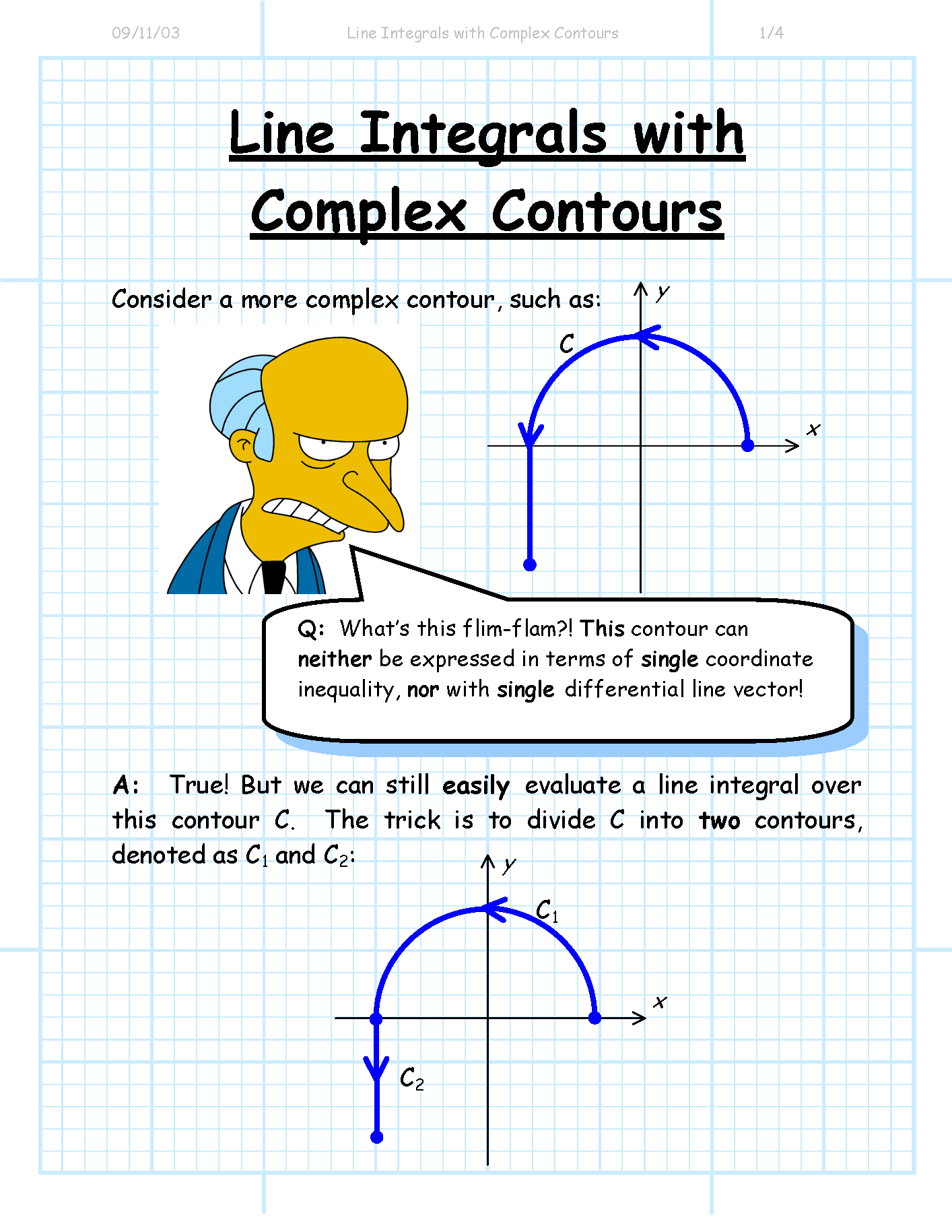
Review Day: Line Integrals

Today we went over several problems involving Line Integrals. We re-emphasized the need to remember how to solve line integrals through other methods that don't involve the fundamental theorem of line integrals. Tomorrow will be the test so there won't be a blog.

What is path independence?



Today in class we went over the implications set forth by the Fundamental Theorem of Line Integrals. For conservative functions, this theorem actual makes otherwise very long problems very easy by simply finding the potential function and then subtracting the function of the beginning point from the function of the end point. We observed that the following are equivalent (refered as T.F.A.E.)

F is conservative <=> F dot dr is path independent <=> Integral over c of F dot dr = 0 for every closed curve

This gives rise to a new integral: a closed-curve (or closed-loop) integral, which can be seen to the left.

We also tested path independence, which is proved by the Fundamental Theorem of Line Integrals: no matter what path you take, the amount of work done is soley based on the beginning and end points (as long as F is conservative)

What is the fundamental Theorem of Line Integrals?

In today's class we explored the implications set forth by the Theorem of Line Integrals, which states that if F(x,y) is conservative and M, N are continuous, then the Integral over C of F dot dr is f(r(b))-f(r(a)) where a<t<b is the bound. What this means is that if the function given is conservative, you can simply find the potential function, then plug in the extreme ends of the bounds in order to evaluate or find work.

One interesting comment that was brought up by Wilson was, can we reverse the direction of piecewise parametrization? Such as going from (1,0) to (0,0) instead of (0,0) to (1,0) in a triangle that goes (0,0) to (1,0), (1,0) to (1,1) and (1, 1) to (0,0)? We will explore this in the next few days, but this led to a larger observance: the direction doesn't matter if the function is conservative and ends up in the same point, work will always be zero.

Here is the inversion seen in the triangle discussed before:

If the function is conservative, the work will be the same for both paths, as long as they both end up at (1,1)

Line Integrals

So on Tuesday, we continued the lesson on line intergrals. A few students (me being one of them) were caught cutting class on Monday. Luckily we weren't punished. At least not yet.
We reviewed the four step process for completing a line integral:
Start with the integral of f (x,y) ds
1) Find a parametric curve, including the limits of the curve
2) Re-parameterize f (x,y) as f (x(t),y(t))
3) Change ds using the arc length formula (which we learned previously)
4) Compute the integral

We also got into the fact that there's a physics aspect to the use of line integrals. (Sigh. Just when I thought I was done with physics)
Let's say you go a path on a 2-D xy coordinate plane with a vector field F (x,y). Think of the vector field as wind that you experience along your "path". We can use line integrals to figure out the net amount of force that is either helping or slowing you down along your "path". It's a cool beginning to the further expansion of line integrals.

     
Note:
The graph of the parametric curve where x (t) = sin (t)
                                                              y (t) = cos (t)
                                                              z (t) = t
 can be described in mutliple ways: a helix, a spring, a slinky, and the list continues on...

How do we compute line integrals?

So the three basic steps to evaluating line integrals is:
1. Figure out the curve C, including limits.
2. Reparameterize F in terms of t.
3. Evaluate.

Sometimes, you may get the same problems with switched x(t) and y(t) values and the answers may have opposite signs of each other. Why? Try drawing out the graph and think about orientation.

Not to say that Mr. Honner didn't teach us enough, but here's a video that might help you practice more with line integrals: http://www.youtube.com/watch?v=fjEvsinvtnw . Ready for that quiz on Friday?

How do we evaluate line/path integrals?

Today we began the lesson by reflecting on parameterization of curves. After such a parameterization, we found the arc length of the same curve. This leads into finding the mass of the curve, which takes both parameterization and arc length into consideration. Quite simply, mass is density times the change in arc length. Refer to the first few problems in the text book (p1069) to practice. More explanation can be found here: http://ocw.mit.edu/courses/mathematics/18-02sc-multivariable-calculus-fall-2010/part-c-parametric-equations-for-curves/

If you are having trouble with some curves, check this out:

This is a new multivariable blogging site that we'll be updating very often about what was learned in class. If you're ever absent, feel free to visit this site to catch up on what we did. We hope this will help you.

On Friday, we learned about flow lines (stream lines). One of the questions in the Utexas homework assignment basically explains what these are: "The flow lines (or streamlines) of a vector field are the paths followed by a particle whose velocity field is the given vector field. Thus, the vectors in a vector field are tangent to the flow lines."

The path of a particle is given by the position function s(t) = < x(t), y(t) >, which are the parametric equations of the flow lines for a vector field F(x,y). You plug them into the separable differential equation dy/dt / dx/dt (or dy/dx) and find its antiderivative after separating all the "x'es" to one side and all the "y's" to another side to get the equation of the flow lines of the vector field. Don't forget to add the constant (C)!

For example, given F(x, y) = < y, x >, find the equation of its flow lines.
dy/dt = x; dx/dt = y --> dy/dx = x/y (separable differential equation)
After separating the "x'es" and "y's," you get ydy = xdx.
Antiderive each side to get ½ y² = ½ x² + C, which is equivalent to y²/2 - x²/2 = C. This is the equation of the given vector field's flow lines. Can you recognize what kind of graph that is?

Hope this was helpful.